By Bob Umlas, Excel MVP

Here we’ll be exploring the various ways to hide and unhide rows and columns in Excel. The bulk of the discussion will address columns, but it applies to rows as well (unless otherwise noted).

How to Hide Columns

You can change a column width by dragging the column separator (the little line between columns) left or right:

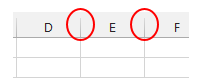
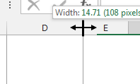
In the following figure, the column separator between D and E is clicked (notice the cursor shape), the mouse is held down, and dragged to the right:

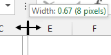
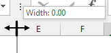
If you drag it to the left enough it will narrow or hide the column (when the width becomes 0 it’s hidden):

When you let go of the mouse there’s a double-line indicating that column D is missing (this shape varies with the version of Excel used):

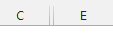
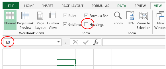
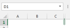
But when headings are not shown (from the View tab you can turn them off), there’s no indication a column is missing. Here, it looks like cell D3 is selected, but in fact it’s E3 because column D is hidden:

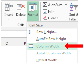
Another way to hide the column is select any cell in the column, say D1, then on the Home tab, in the Cells group, there’s a Format dropdown which has access to the Column Width:

When you issue the command, you get a dialog with the current width, like this:

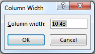
You can type in any number from 0 to 255, however when you type 0 the column is hidden.

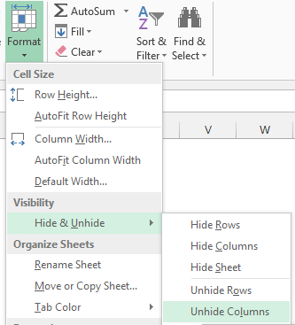
You can also hide a column via Home/Format/Hide & Unhide/Hide Columns.

There’s also a shortcut to hide a column. Whichever column is selected will become hidden when you press ctrl/0 (a row will hide when you press ctrl/9).

All of the above applies to more than one column as well. If you select A1:E1 and use any of the methods, all 5 columns will hide.

How to Unhide Columns

Okay, how about unhide a cell? Again, there are several ways. It’s not as easy to select a hidden column, however! So you can type the cell address into the name box to get the cursor into the column. Or, you can press the F5 key (Go To) and type in the cell address. Here, D1 was entered into the name box:

The cell D1 became selected. You can unhide this with the column width command we saw above, change the 0 which will be there to 8.43, or any number, etc. This is not literally an unhidden cell– it’s resetting the column width to a number. When you unhide, it will restore the width to what it was before it was hidden! You can unhide it by Home/Format/Hide & Unhide/Unhide Columns:

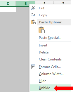
Ctrl/shift/0 (ctrl/shift/9 to unhide rows) will do the job as well. You can also select the columns before and after the hidden column and unhide them (only the hidden one will be affected). Here, C thru E is selected:

And finally, you can carefully position the cursor a little to the right of the D-column separator so it looks something like this:

then drag to the right which will reveal column D!

Lastly, suppose you have text like this:

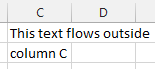
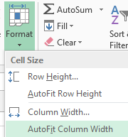
And you want to widen column C so it all fits. There are a few ways to do this. You can drag the column separator between C and D to the right and visually adjust it. You can double-click the column separator which does a “best-fit” for the longest cell in that column. Or you can select a few cells (vertically or horizontally) or the entire column, and use Home/Format/AutoFit Column Width:

Enjoy!

Learn more about IIL’s Microsoft Excel training >>

Bob Umlas has been voted an “MVP” (Most Valuable Professional) by Microsoft each year since 1994 for his contributions to Excel online forums and he is known world-wide for his expertise. As an MVP, he meets yearly with fellow MVPs at Microsoft’s headquarters in Redmond, where he has access to the product developers. He has also been a beta tester for new versions of Excel since version 1.5 and is the author of several books including This isn’t Excel, it’s Magic! (available on the IIL Bookstore), Excel Outside the Box, and More Excel Outside the Box.