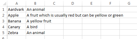
Using VLOOKUP in Excel seems to be a mystery to many. But you do it all the time in real life—you look up a word in a dictionary and scan a little to the right to read the definition. Well, it could be the same thing in Excel:
If you wanted to use Excel to look up a word in this dictionary, the syntax would look something like this:
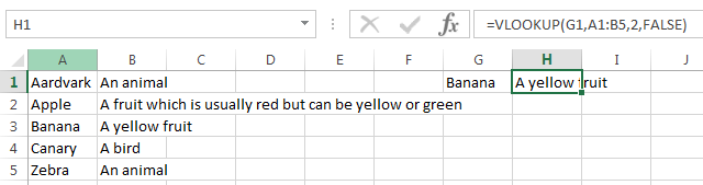
The syntax is =VLOOKUP(what,where,returning which column,approximate match?)
“What” you’re looking up is cell G1, or Banana.
“Where” you’re looking it up is in the dictionary which is A1 thru B5 (A1:B5)
“Returning which column” is from the second column, or 2 (not “B”, because Excel’s syntax requires a number, not a letter).
“Approximate Match” is FALSE because we want an exact match.
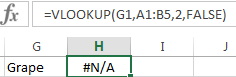
Let’s say I looked up “Grape” in this dictionary:
The #N/A indicates it’s “Not Available”. Therefore “Grape” is not in this dictionary.
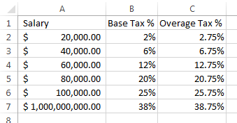
You may be wondering, “Why would anyone want an approximate match?” Well, suppose you’re looking up your salary in a tax table, and suppose you make $75,000. Here’s the fictitious table:
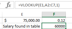
Your $75,000 isn’t in the table. It would be wrong here to get a #N/A error! You do owe taxes! You owe 12% of the first $60,000, and 12.75% of anything over that. So we’d use the TRUE instead of FALSE in the VLOOKUP formula (Since it’s assumed TRUE if omitted, we can just omit it):
The .12 is the 12% found next to the $60,000 item (cell B4) because we didn’t ask for an exact match. (When you do ask for the approximate match, the lookup column must be in sequence). Note that Excel does not also pick up the formatting, so the 12% is shown as .12. The value is the same, of course. Also note that the range we’re looking at is A2:C7 – we don’t include the headings in row 1.
In the following figure, we see that the 12% is for the first $60,000, so we need to “find” that $60,000:
Then these 2 values in column F need to be multiplied together to get the base tax amount:
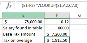
The remaining part is to find the amount over the $60,000, then the tax on that overage. This is seen here:
This is a little trickier as we’re looking at a few calculations simultaneously. The difference is E1 minus F2; the $75,000 less the $60,000. This is places in parentheses so we can multiply that difference by the tax found in the 3rd column, the VLOOKUP(E1,A2:C7,3). This gives the result of $1912.50.
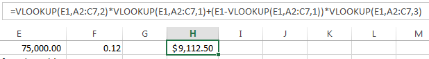
The total tax can now be found by adding the overage to the base:
For you adventurous folks, here’s the same answer all done in one cell:
A few final notes:
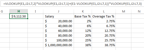
If the table started in column J, the column reference would still be 1, 2, or 3, not 10, 11, and 12, (the column number for J, K, and L) because the formula is looking for the relative column in the range. The above formula would be:
Bob Umlas has been using Excel since version 0.99 (on the Macintosh)! He was a contributing editor to Inside Microsoft Excel for many years. He has had more than 300 articles published on subjects ranging from beginner to advanced macros, and on tips, shortcuts, and general techniques using virtually all aspects of Excel.
He was voted an “MVP” (Most Valuable Professional) by Microsoft each year from 1993-2018 (25 years!) for his contributions to the various online Forums about Excel and is known world-wide for his contributions in Excel. He is the author of “This isn’t Excel, it’s Magic!” which is available from http://www.iil.com/publishing as well as from Amazon.com. He has had more than 300 articles published on subjects ranging from beginner to advanced macros, and on tips, shortcuts, and general techniques using virtually all aspects of Excel.
From 1998 to 2018 Bob worked for a major tax and accounting firm, using Microsoft Excel® 8 hours a day, writing custom applications for staff and clients.