Excel Grand Totals: You DON’T Need Long Formulas
By Bob Umlas, Excel MVP
February 24, 2016
Still using long formulas to create grand totals in Excel? There is a better way!
Suppose you have a worksheet which looks something like this:

Clearly, what’s needed is the grand total in cell B38. Notice that there are several subtotals in the list. The formula in cell B9, for example, is =SUM(B4:B8).
How many of you would use the formula =B3+B9+B14+B20+B25+B32+B37 to solve the problem?

I’ve seen formulas like this many many times, and often a lot longer because the list is longer. It does work, producing the correct answer, but it’s tedious to do and certainly subject to errors because you might click the wrong cell.
In this blog I’ll describe a few alternative ways to do this, leaving the best for last!
The first way is probably the easiest, but the formula is perhaps just as long. While the cell B38 is selected, press Alt/= (that is, hold the Alt key down and press the = sign). This creates this formula:

Wow! That’s cool! Excel “finds” all the other Sum formulas and picks out the correct cells! Not likely to produce an error! But there’s no hunting for the correct cells to use. One down side to this technique is that it won’t work on a range which is horizontal, only vertical, as this one is.
Let’s look at some shorter ones:

This doesn’t look much shorter, but it’s pretty much the same size no matter how many cells are involved. So it’s definitely shorter than something like
=B1+B6+B11+B17+B20+B26+B32+B37+B40+B44+B50+B54+B60+B66+B81+B90+B99+B106+B112+B121+B126+B130+B134+B154+B159+B144+B176+B188+B192+B198+B206
!!
And I’ve seen longer! (4 lines worth!)
OK, what is SUMIF? It’s a built-in Excel function which works like this: Wherever the first range (A1:A37) contains the word “Subtotal”, add the values from the 2nd range (the 3rd parameter). The actual syntax is:

That’s pretty cool too! But this could also lead to an error if somewhere in column A the word Subtotal were misspelled, or contained a space at the end (“Subtotal ”)!
OK, ready for the winner? Make sure you’re sitting down first.
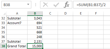
How about =SUM(B1:B37)/2:

What? How can that work?
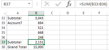
Well, let’s look at the formula in B37, for example:

That’s adding up the values in B33:B36. Those values total 2,131. If I add the values in B33 thru B37 (including the subtotal), I get 4,262 – the 2,131 from B33:B36 and the same 2,131 from B37. So I’m adding the values in twice! So if I divide by 2, I get the right answer! Each of the sections containing the subtotal had the values in there twice – the individual values plus the subtotal! So dividing by 2 solves the problem!
This makes the technique work horizontally as well, using a formula something like =SUM(A2:AK2)/2.
Here’s the same data we were looking at, but turned on its side:

Clearly, we get the same answer! No more lonnnngggggg formulas to do this task!
Bob Umlas
Bob Umlas has been voted an “MVP” (Most Valuable Professional) by Microsoft each year since 1994 for his contributions to Excel online forums and he is known world-wide for his expertise. As an MVP, he meets yearly with fellow MVPs at Microsoft’s headquarters in Redmond, where he has access to the product developers. He has also been a beta tester for new versions of Excel since version 1.5 and is the author of several books including This isn’t Excel, it’s Magic! (available on the IIL Bookstore), Excel Outside the Box, and More Excel Outside the Box.


